Tag Archives: math programming

March 18, 2014

creating a March Madness bracket using integer programming

An Associated Press article on ESPN outlines how the Division I men’s basketball committee wants to make bracket construction to be more fair [Link]. At present, there are 68 teams with no plans to expand the field. However, the committee has many decisions to make when it comes to who makes it in and who doesn’t as well as the seed and the region. All of this together determines potential matches. Previously, the committee tried to entirely avoid rematches in the first few rounds of the tournament. Given the large number of potential match-ups depending on who wins and loses, this constrained the bracket (possibly too much).

“There have been years where we’ve had to drop a team or promote a team; there was even a year where teams dropped two seed lines. We don’t feel that’s appropriate.” – Ron Wellman, the athletic director at Wake Forest

The article doesn’t exactly hint that integer programming could be used to solve this problem, but that’s the next logical step. In fact, there is a paper on this! Cole Smith, Barbara Fraticelli, and Chase Rainwater developed a mixed integer programming model (published in 2006, back when there were 65 teams) to assign teams to seeds, regions, and pods (locations). The last issue is important: constructing the bracket is intertwined with assigning the bracket to locations for play. For example, four teams in a region in the field of 64 (e.g., a 1, 8, 9, and 16 seeds) must all play at the same location to produce a single team in the Sweet 16.

The Smith et al. model minimizes the sum of the (then) ﬁrst-round travel costs (the round of 64), the (then) expected second-round travel costs (the round of 32), and the reseeding penalty costs while considering typical assignment constraints as well as several side constraints, including:

no team plays on its home court (except in the Final Four – that location is selected before the tournament),
no intra-conference match-ups occur before the regional ﬁnals (what was the fourth round). This is the constraint that may be relaxed somewhat in the new system. Therefore, this existing model can be used to make brackets in the proposed new system.
the top-seeded team from each conference must be assigned to a different region as the second- and third-highest seeded teams from that conference.
the best-seeded teams should be assigned to nearby pods (locations) in the ﬁrst weekend (a reward for a good season!), and
certain universities with religious restrictions must be obeyed (e.g., Brigham Young University cannot play on Sundays).

It is worth pointing out that this model assigns the seeds to teams. A team that could be considered as an 11-13 seed would be assigned its seed (11, 12, or 13) based on the total cost of the system. That may seem like it’s unfair on some level, but it might be better for a team to be a 13 seed and play nearby than a 12 seed but have to travel an extra 1000 miles. (Note: Nate Silver and the 538 team use travel distance in their NCAA basketball tournament prediction model because distance matters). Flexible seeds allows for a bracket that gives more teams a fair shot at winning their games, but too much flexibility would be unfair to teams. The Smith et al. model allows for some flexibility for 6-11 seeds.

The mixed integer programming model by Cole Smith, Barbara Fraticelli, and Chase Rainwater already addresses the committee’s concerns, which begs the question: why isn’t the committee using integer programming??

OK, it’s probably pretty easy to think of a few reasons, and none of them involve math. One concern is that the general public seems to distrust models of any kind. This may be because models are black boxes to non-experts. This lack of transparency makes it hard to generate any kind of public support (Exhibit A: the debate about the model for the BCS football rankings). Perhaps marketing could improve buy in (“The average team traveled 500 miles fewer this year than last” or “Five teams had to travel across all four US time zones last year, and none had to do so this year.”) A better suggestion may be to give a few of the top integer programming solutions to the committee, who can then use and adapt (or ignore) the solutions as they see fit. Currently, the committee looks at several rankings (including the LRMC method, last time I heard), so they are already using math models to influence the decisions ultimately made by humans.

How would you use operations research and math modeling to improve the tournament selection and seeding process?

Reference:

Smith, J.C., Fraticelli, B.M.P, and Rainwater, C., “A Bracket Assignment Problem for the NCAA Men’s Basketball Tournament,” International Transactions in Operational Research, 13 (3), 253-271, 2006. [Link to journal site]

Leave a comment | tags: march madness, math programming | posted in Uncategorized

July 25, 2013

mixed integer programming myth of the day: checking for feasibility

By Laura Albert

This is the third post in my MIP 2013 series on mixed integer programming myths and counterexamples. See my first two posts here and here. Again, the Myths are from the excellent “Myths and Counterexamples in Math Programming” in the Mathematical Programming Glossary.

Today’s MIP Myth (#22) is as follows: For any 0-1 integer program with a single constraint, there is a branch-and-bound algorithm that can determine if the 0-1 integer program has a feasible solution in polynomial time.

Read about branch-and-bound (B&B) here. The idea is that a linear programming model is solved, and if the solution has variables with fractional values, a tree is created that branches on one of the fractional variables. For binary variables considered here, one branch would set the variable in question to 0 and the other branch would set the variable equal to 1. In the worst case, the tree has depth n, where n is the number of variables, which leads to a tree with an exponential number of nodes.

The myth here explores whether it is possible to quickly check to see if the integer program admits any feasible solution up front. Quick here means in polynomial time. This can be achieved without having to create the entire B&B tree with its exponential size. To show that checking for feasibility sometimes requires exponential time, consider the following IP:

$\max x_1 :\ x \in \{0,1\}^n,\ 2 x_1 + 2 x_2 + ... + 2 x_n = n.$

From inspection, we can see that there no feasible solutions if n is odd. If n is even, there are many feasible solutions. (Note: there is a lot of symmetry in this IP).

Jeroslow (1974) shows that for any fixed values of the fractional variables in the linear programming relaxation, one must evaluate at least $2^{\lceil n/2 \rceil}$ nodes before it certifies that it is infeasible (not polynomial time). The paper is very short and provides the proof (see the reference below).

The following note was in the “Myths and Counterexamples in Math Programming”:

Ed Klotz points out that modern B&B algorithms are more broadly construed to include preprocessing, among other things, that would solve this example without exhaustive search. The counterexample does emphasize the need for such things.

Reference:
RG Jeroslow, 1974. Trivial integer programs unsolvable by branch-and-bound, Mathematical Programming 6(1), 105-109.

2 Comments | tags: math programming, mip | posted in Uncategorized

July 24, 2013

mixed integer programming myth of the day: problems vs. models

By Laura Albert

This is the second post in my MIP 2013 series on mixed integer programming myths and counterexamples. See my first post here. Again, the Myths are from the excellent “Myths and Counterexamples in Math Programming” in the Mathematical Programming Glossary.

Today’s MIP Myth (#16) is as follows: Alternative optima in a MIP model correspond to equally good problem solutions.

I like this myth because it addresses the difference between the problem and the model. We assume they are the same, but they are not. Additionally, there may be multiple ways to model the same problem.

Consider the TSP (a problem!). Here is one IP for the TSP:

$\min \sum_{i,j} c_{ij} x_{ij} : x \in \{0,1\}^{n \times n}$
$\sum_i x_{ij} = 1, \ \forall j,\ \sum_j x_{ij} = 1, \ \forall i$
$\sum_{(i,j) \in S} x_{ij} \le |S|-1,\ \forall S : \emptyset \neq S \subset \{1,...,n\}$

Here, the variables $x_{ij}=1$ if node j is visited after node i. The c values are the costs/distances. Assume that c is symmetric here. The second line makes sure that each city/node is visited once. The last line shows the subtour elimination constraints.

There are several alternative optima that are not equally good alternative problem solutions; they are the same solutions. Let’s assume that there is a single tour in the problem that optimizes the objective function. Here, notice that with symmetric costs, it doesn’t matter if we traverse this tour forward or backward. In the model, this single optimal solution can be represented by two solutions that have the same objective function value (starting with node 1):

$x^* = \{1,2,...,n-1,n,1\}$

$x' = \{1,n,n-1,...,2,1\}$ .
with
$x'_{ij}=1$ if $x^*_{ji}=1$ and 0 otherwise.

Here is a picture of these two tours.

These two TSP tours are the same solution illustrated forward and backward.

There are other ways to model the TSP. One involves defining the variables as:
$x_{ik} = 1$ if node i is the kth node in the tour and 0 otherwise. Parts of the IP model above would have to be reformulated, but I’ll omit that here. There are n identical solutions (2n if the costs are symmetric). The following two tours are different solutions to the model that are the same tour in the problem:

$\{1,2,...,n-1,n\}$
$\{2,3,...,n-1,n,1\}$
and so on.

This issue is called symmetry in integer programs, where you can relabel the vertices, rotate the problem, perform a rigid transformation, etc. and have the same solution with a different representation of the variables. It can really slow down solver/algorithm performance, which is why some people work on breaking symmetry.

I liked finding this myth because it’s practical, important to know, and something I haven’t done a good job at conveying to students. I’ll be sure to do a better job in the future.

Comments are welcome!

1 Comment | tags: math programming, mip | posted in Uncategorized

July 23, 2013

mixed integer programming myth of the day

By Laura Albert

I am attending MIP 2013 in Madison, Wisconsin this week. In honor of mixed integer programming, I am going to blog about one MIP myth every day during the conference. The Myths are from the excellent “Myths and Counterexamples in Math Programming” in the Mathematical Programming Glossary.

Today’s MIP Myth is as follows: If an integer linear program has an unbounded linear programming relaxation, the integer linear program is also unbounded.

The following counterexample is due to Byrd, Goldman, and Heller [1987], which is based on Meyer [1974], who showed this cannot happen with rational data and a feasible integer linear program.

The counterexample uses irrational data. Here is the IP model:

$\max x_1 : x \ge 0,\ x \in Z^4,\ x_3 - \sqrt{2} (x_1 - x_2) = 0,\ x_2 + x_4 = 1$

With linear variables, the objective is maximized as $x_1 \rightarrow \infty$ . In fact, the LP relaxation contains the ray 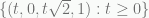$\{(t, 0, t \sqrt{2}, 1) : t \ge 0\}$ . Therefore, the LP relaxation is unbounded.

Let’s take a look at this problem with integer variables. The first constraint (rearranged yields $x_3 = \sqrt{2} (x_1 - x_2)$ ) can only happy when both sides are zero for integer variables. Therefore, we know that $x_1 = x_2 = 0$ or $x_1 = x_2 = 1$ and that $x_3 = 0$ in either case. Putting this together, there are only two feasible points in the integer programming model: (0, 0, 0, 1) and (1, 1, 0, 0). As you can see, it is not unbounded.