Tag Archives: mip

July 25, 2013

mixed integer programming myth of the day: checking for feasibility

This is the third post in my MIP 2013 series on mixed integer programming myths and counterexamples. See my first two posts here and here. Again, the Myths are from the excellent “Myths and Counterexamples in Math Programming” in the Mathematical Programming Glossary.

Today’s MIP Myth (#22) is as follows: For any 0-1 integer program with a single constraint, there is a branch-and-bound algorithm that can determine if the 0-1 integer program has a feasible solution in polynomial time.

Read about branch-and-bound (B&B) here. The idea is that a linear programming model is solved, and if the solution has variables with fractional values, a tree is created that branches on one of the fractional variables. For binary variables considered here, one branch would set the variable in question to 0 and the other branch would set the variable equal to 1. In the worst case, the tree has depth n, where n is the number of variables, which leads to a tree with an exponential number of nodes.

The myth here explores whether it is possible to quickly check to see if the integer program admits any feasible solution up front. Quick here means in polynomial time. This can be achieved without having to create the entire B&B tree with its exponential size. To show that checking for feasibility sometimes requires exponential time, consider the following IP:

$\max x_1 :\ x \in \{0,1\}^n,\ 2 x_1 + 2 x_2 + ... + 2 x_n = n.$

From inspection, we can see that there no feasible solutions if n is odd. If n is even, there are many feasible solutions. (Note: there is a lot of symmetry in this IP).

Jeroslow (1974) shows that for any fixed values of the fractional variables in the linear programming relaxation, one must evaluate at least $2^{\lceil n/2 \rceil}$ nodes before it certifies that it is infeasible (not polynomial time). The paper is very short and provides the proof (see the reference below).

The following note was in the “Myths and Counterexamples in Math Programming”:

Ed Klotz points out that modern B&B algorithms are more broadly construed to include preprocessing, among other things, that would solve this example without exhaustive search. The counterexample does emphasize the need for such things.

Reference:
RG Jeroslow, 1974. Trivial integer programs unsolvable by branch-and-bound, Mathematical Programming 6(1), 105-109.

2 Comments | tags: math programming, mip | posted in Uncategorized

July 24, 2013

mixed integer programming myth of the day: problems vs. models

By Laura Albert

This is the second post in my MIP 2013 series on mixed integer programming myths and counterexamples. See my first post here. Again, the Myths are from the excellent “Myths and Counterexamples in Math Programming” in the Mathematical Programming Glossary.

Today’s MIP Myth (#16) is as follows: Alternative optima in a MIP model correspond to equally good problem solutions.

I like this myth because it addresses the difference between the problem and the model. We assume they are the same, but they are not. Additionally, there may be multiple ways to model the same problem.

Consider the TSP (a problem!). Here is one IP for the TSP:

$\min \sum_{i,j} c_{ij} x_{ij} : x \in \{0,1\}^{n \times n}$
$\sum_i x_{ij} = 1, \ \forall j,\ \sum_j x_{ij} = 1, \ \forall i$
$\sum_{(i,j) \in S} x_{ij} \le |S|-1,\ \forall S : \emptyset \neq S \subset \{1,...,n\}$

Here, the variables $x_{ij}=1$ if node j is visited after node i. The c values are the costs/distances. Assume that c is symmetric here. The second line makes sure that each city/node is visited once. The last line shows the subtour elimination constraints.

There are several alternative optima that are not equally good alternative problem solutions; they are the same solutions. Let’s assume that there is a single tour in the problem that optimizes the objective function. Here, notice that with symmetric costs, it doesn’t matter if we traverse this tour forward or backward. In the model, this single optimal solution can be represented by two solutions that have the same objective function value (starting with node 1):

$x^* = \{1,2,...,n-1,n,1\}$

$x' = \{1,n,n-1,...,2,1\}$ .
with
$x'_{ij}=1$ if $x^*_{ji}=1$ and 0 otherwise.

Here is a picture of these two tours.

These two TSP tours are the same solution illustrated forward and backward.

There are other ways to model the TSP. One involves defining the variables as:
$x_{ik} = 1$ if node i is the kth node in the tour and 0 otherwise. Parts of the IP model above would have to be reformulated, but I’ll omit that here. There are n identical solutions (2n if the costs are symmetric). The following two tours are different solutions to the model that are the same tour in the problem:

$\{1,2,...,n-1,n\}$
$\{2,3,...,n-1,n,1\}$
and so on.

This issue is called symmetry in integer programs, where you can relabel the vertices, rotate the problem, perform a rigid transformation, etc. and have the same solution with a different representation of the variables. It can really slow down solver/algorithm performance, which is why some people work on breaking symmetry.

I liked finding this myth because it’s practical, important to know, and something I haven’t done a good job at conveying to students. I’ll be sure to do a better job in the future.

Comments are welcome!

1 Comment | tags: math programming, mip | posted in Uncategorized

July 23, 2013

mixed integer programming myth of the day

By Laura Albert

I am attending MIP 2013 in Madison, Wisconsin this week. In honor of mixed integer programming, I am going to blog about one MIP myth every day during the conference. The Myths are from the excellent “Myths and Counterexamples in Math Programming” in the Mathematical Programming Glossary.

Today’s MIP Myth is as follows: If an integer linear program has an unbounded linear programming relaxation, the integer linear program is also unbounded.

The following counterexample is due to Byrd, Goldman, and Heller [1987], which is based on Meyer [1974], who showed this cannot happen with rational data and a feasible integer linear program.

The counterexample uses irrational data. Here is the IP model:

$\max x_1 : x \ge 0,\ x \in Z^4,\ x_3 - \sqrt{2} (x_1 - x_2) = 0,\ x_2 + x_4 = 1$

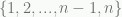
With linear variables, the objective is maximized as $x_1 \rightarrow \infty$ . In fact, the LP relaxation contains the ray $\{(t, 0, t \sqrt{2}, 1) : t \ge 0\}$ . Therefore, the LP relaxation is unbounded.

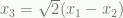Let’s take a look at this problem with integer variables. The first constraint (rearranged yields $x_3 = \sqrt{2} (x_1 - x_2)$ ) can only happy when both sides are zero for integer variables. Therefore, we know that $x_1 = x_2 = 0$ or $x_1 = x_2 = 1$ and that $x_3 = 0$ in either case. Putting this together, there are only two feasible points in the integer programming model: (0, 0, 0, 1) and (1, 1, 0, 0). As you can see, it is not unbounded.