Tag Archives: sports

What analytics really say about when to go for a two point conversion in an NFL game

The two point conversion has become more popular in National Football League (NFL) games, and it has become a popular topic of conversation in the NFL playoffs leading up to the Super Bowl. I once wrote a blog post that uses dynamic programming to identify when to go for 2 based on the score differential and the number of possessions remaining in the game. The analysis also shows what difference the choice makes, noting that most of the time the win probability does not make a huge difference in the outcome of the game, affecting the win probability by less than one-percent in most cases. In this post, I delve into the two point conversion, covering rule changes, football strategy, and assumptions.

By the numbers

In 2023, a typical NFL team attempted a two-point conversion about once 1 every 4 games and was successful just over half the time. A decade ago, a typical team attempted a two-point conversion about once 1 every 8 games and was successful just under half the time. Two point conversions became more popular and more successful. Two rule changes influenced these changes:

  1. In 2015, the NFL moved the extra point attempt from the 2 yard line to the 15 yard line.
    • The proportion of extra points that succeeded lowered from 0.996 (in 2015) to 0.941 in the seasons after the change. A chart in an article on Axios illustrates how dramatic this change has been on extra point success rates.
  2. In 2023, a new rule allowed offenses to attempt a two point conversion from the 1 yard line (instead of the 2 yard line) when there was a defensive penalty on a touchdown.
    • The proportion of two point conversions that succeeded increased from about 0.5 to 0.565, the first season the success rate was well-above 0.5.

The difference of one yard makes a difference. For comparison, attempts to go for it on fourth down and two yards to go succeed 57.2% of the time, and this increases to 65.5% for fourth down and one yard to go.

Decision-making

After a team scores a touchdown, they have essentially two choices. They can kick an extra point or they can attempt a two point conversion. The proportion of extra point attempts that were successful in 2023 was 0.96, and historically the proportion of two-point conversions that have been successful is 0.48. Therefore, on average, the extra point attempt or two-point conversion have promised roughly the same number of points on average.

The goal is not to maximize expected points, it’s to win the game. The two rule changes above have tipped decision-making in favor of the two point conversion in more situations by making the extra point attempt less attractive and the two point conversion more attractive.

The “best” choice for improving the chance of winning is situational and depends on a few factors:

  • Point differential
  • Time remaining (including time outs remaining)
  • Strategies that each team may employ in the resulting situations
  • Specific teams and match-ups

The dynamic programming model takes the first two factors into account, where the time remaining is modeled as the number of possessions remaining. Dynamic programming is an algorithmic approach that essentially enumerates the possible outcomes of the remaining drives in the game to quantitively determine the best options for the average team. This approach does not take specific situations into consideration, however, it is informative as a baseline.

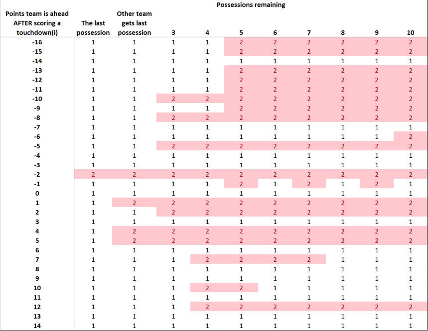
Using 2023 data, I present a chart of when the average team should attempt a two-point conversion based on the 2023 data. In this chart, pictured below, the rows capture the point differential when a touchdown is scored, with a negative score capturing how many points a team is behind. The columns capture how many possessions are remaining in the game, including the current possession. Therefore, as the game evolves, we move left in the table. The team with the final possession of the game has 1 possession remaining in the table, and a team with two possessions left will not get the ball back. Note that there are 22.2 total possessions per game, on average, so the last 6 possessions or so capture the fourth quarter.

Table 1: when an average team should choose to go for a two point conversion after scoring a touchdown based on the score differential and number of remaining possessions [2023 data]

According to this chart, an average team should attempt a two point conversion in many situations, including when a touchdown in the fourth quarter puts the team down by 8, 5, 2, or 1 or up by 1, 2, 4, 5, and 7. A team should not go for two when a touchdown puts the team down by 4 or 3, puts the team up by 3 or 6, or ties the game.

Compared to 2014–before the two rule changes mentioned above–two point conversations are now the better choice in more situations. For example, a two point conversation now is the better choice for the average team when a touchdown in the fourth quarter puts the team down by 1.

My analysis, as Prof. Ben Recht notes in an outstanding post on two point conversions, makes a number of assumptions. While some assumptions are more reasonable than others, the model still offers important insights that are not obvious before crunching the numbers.

A better way to decide whether to attempt a two point conversion

When I listen to broadcasts, I get frustrated with the analytics discourse from the commentators, which is often some version of “The analytics tell you to go for 2 in this situation.”

This is wrong. Analytics do not tell people what to do. Analytics are a collection of tools that can inform decision-making, with people making the final decisions.

If I were a football coach, I would not use the chart above. I would ask for a different chart based on the same analysis. Below, I create this chart.

No team is the average team. As noted earlier, the analysis using dynamic programming makes some assumptions that are not totally valid, including that an average team is facing an average team. The chart above always gives the same answer for the same point differential and possessions remaining, and it does not reflect other attributes of the situation at hand.

One specific situation that may affect the decision is the play that a team has available for the two point conversion. For example, historically 43.4% of pass plays have succeeded, whereas 61.7% of run plays have succeeded. Having a play in mind–and its associated likelihood of success–should affect the decision. Another situation is the team’s opponent, including their run and pass defense.

There are two ways to make the dynamic programming more informative for specific situations:

  1. Change the inputs to reflect the current match-up. In this case, one could change the probability that a two point conversion would be successful, the probability that an extra point is successful, the probability that a drive ends in a touchdown, and the probability that a drive ends in a field goal.
  2. Instead of only reporting the best decision (go for 1 or go for 2), the analysis can be used to report the probability that a two point conversion should be successful for it to be the better choice than attempting an extra point. In this case, a decision-maker (a football coach) can estimate how likely their play would success against the team they are playing in the specific situation they are facing.

I illustrate the second approach below using the dynamic programming analysis above. Instead of reported the binary decision of going for 1 or 2 as before, I report the two point conversion probability of success above which going for two is the better decision. Again, I use data based on average teams. The lower the probability in the chart, the more attractive the two point conversion is.

Some decisions are clear cut. A 0.00 indicates that a team should always go for a two point conversion, and a 0.95 indicates that a team should essentially always attempt the extra point. Most of the probabilities are in between, which means that the “best” decision is not clear cut in most cases.

Table 2: the minimum probability of success associated with a two point conversion above which going for 2 is the better decision based on the score differential and number of remaining possessions. Situations that always result in a loss or a win are labeled “Lose” and “Win,” respectively [2023 data]

This new chart is more nuanced than the first chart in this post.

  • Sometimes it is obvious to go for 2. A two point conversion is the better decision with a play that has a mere 25% probability of success when a touchdown in the fourth quarter puts the team down by 10, 5, or 2, or up by 1 or 5.
  • Sometimes it is obvious to attempt an extra point. Going for two is the better decision with a play with a very high, 75% probability of success, which occurs when a touchdown puts a team down 7 or 3, up 3 or 8, or ties the game. Very few plays can expect a 75% probability of success, so in these situations it almost always is better to attempt the extra point.

Now consider strategies for two different teams:

  • Team A with a two point conversion play with a 40% probability of success, and
  • Team B with a two point conversion play with a 60% probability of success.

Team A and Team B would make different decisions if a touchdown in the fourth quarter puts them down by 9, 6, 4 or up by 3, 6, or 7.

Another insight: Both Team A and Team B should both attempt a two point conversion if a touchdown puts them down by 8.

Therefore, the same chart yields different “best” solutions for different teams based on the situations at hand. This insight follows directly from the numbers and the modeling, however, it is almost always overlooked in discussions on football analytics.

Related articles and posts:


the mathematics of rare matchups in the March Madness tournament

This year’s Final Four is set in the NCAA men’s basketball tournament, with Duke, the University of North Carolina (UNC), Kansas, and Villanova facing off this weekend. This is the first time Duke and UNC will play in the tournament. At first blush this is hard to believe when considering how often these two teams have played in the tournament (a combined total of 334 games!). It’s easier to believe when considering the mathematics used to create the bracket.

I once blogged about the constraints required to seed the 68 teams in the tournament and build the bracket. The NCAA’s website indicates the same rules are still in use.

First, the 68 teams are selected, sorted, and seeded. This is a long process. Then, the 68 teams are assigned to one of the four regions to create the bracket. There are many rules for this last step. Here is the rule that explains why Duke and UNC haven’t played in the tournament before:

“Each of the first four teams selected from a conference shall be placed in different regions if they are seeded on the first four lines.”

https://www.ncaa.com/news/basketball-men/article/2021-01-15/how-field-68-teams-picked-march-madness

Duke and UNC are almost always in the first four teams of their conference, the Atlantic Coast Conference. They typically play each other twice during the regular season and sometimes a third time in the ACC conference tournament. Duke and UNC played each other twice this season. According to the NCAA constraints for constructing a bracket, Duke and UNC are not allowed to meet in the tournament before the Final Four. This is when they are meeting in the 2022 tournament. Mathematical constraints secretly guide the tournament.

Fun fact: it is not always possible to create a feasible bracket that conforms to all of the rules.

There are several other constraints for constructing a bracket. Infeasibility can happen in real applications of mathematical optimization. Mathematical constraints do not make nuanced exceptions to the rules the way human decision makers do, so infeasible problem instances must be addressed with humans.

The selection committee addresses the problem of infeasibility by moving a team’s seed up or down by one and sometimes two. This seems like a small change, but it can drastically change a team’s path to the Final Four. The good news is that about a decade ago the rules were tweaked to change teams’ seeds less often, in a victory for the tournament and also for mathematics.


The Packers should have gone for it on 4th and goal

The Green Bay Packers were defeated by the Tampa Bay Buccaneers last night. The Packers trailed 31-23 when it was fourth down and goal with 2:22 to go in the fourth quarter. The Packers decided to kick a field goal instead of trying for a touchdown. The decision was universally criticized. Without crunching the numbers, I knew it would be better to go for it and attempt to get a touchdown, even though either decision was a longshot. The Packers lost 31-26.

Since the game ended, I crunched the numbers.

Here is how I approached the decision. First, the Packers needed a series of events to occur, with all or nearly all events working in their favor to win. Computing the probability of the intersection of multiple events occurring is likely to be a small number. I examined the pathways to winning below. There were some fluke ways to win that I left out because those probabilities were negligible. My calculations are in this spreadsheet.

Decision #1: Go for it on fourth down. There are two ways to win in this scenario.

  1. Score a touchdown.
  2. Make the two point conversion to tie the game.
  3. Stop the Buccaneers defensively (a TB field goal means the Packers lose).
  4. Win by scoring within regulation or in overtime if time expires.

I estimate that the Packers had a probability of 0.6 of scoring a touchdown based on Aaron Rodgers’s pass completion numbers. Teams have a probability of 0.48 of getting the two point conversion. Teams have a probability of 0.68 of stopping their opponent from scoring on a possession. There was not much time on the clock, so this may have been an underestimate. However, both teams had multiple time out to stop the clock, and there had not yet been the two minute warning. Winning in overtime for two evenly matched teams is 50-50. Winning within regulation with very little time left has a small probability (say, 0.03). Putting this together, I estimate that the Packers had a win probability of 0.104.

Decision #2: Make a field goal attempt. There are also two ways to win in this scenario:

  1. Make the field goal.
  2. Stop the Buccaneers defensively while leaving enough time on the clock to score.
  3. Win by scoring a touchdown within regulation.

or

  1. Miss the field goal.
  2. Stop the Buccaneers defensively while leaving enough time on the clock to score.
  3. Score a touchdown within regulation, make the two point conversion to tie, and win in overtime (see Decision #1).

I estimate that the Packers had a probability of 0.96 of scoring a field goal. Teams normally have a probability of 0.68 of stopping their opponent from scoring, but I lowered that to 0.5 here because it needed to happen in such a way that the Packers had enough time for one last drive. That is likely an optimistic estimate. I estimate that the Packers could score a touchdown with a probability of 0.15 with the remaining time (Rodgers had an MVP worthy season). The second way to win involved missing the field goal and tying the game in regulation with a last second touchdown and later winning in overtime. Putting this together, I estimate that the Packers had a probability of 0.076. I believe this is optimistic.

Takeaways

  1. Going for a touchdown increasing the win probability by about 3% compared to kicking a field goal. It’s not a huge different, but it’s also not insignificant.
  2. Either way, the Packers were unlikely to win. So while the decision was bad, it wasn’t a decision that likely cost the Packers the game.
  3. Kicking the field goal (Decision #2) could make sense with high confidence in a defensive stop or scoring a TD with time expiring. For the best defensive team in the NFL, decision #2 might be the better option. If Tampa Bay had, say, the worst defense in the country, especially if their secondary was weak, Decision #2 would be more attractive.
  4. The Packers had two bad choices.

a soccer win probability model

Last year, I tweeted about a win probability model I created for soccer (or football, depending on where you are from) and the 2019 FIFA Women’s World Cup case study. I promised to blog about this case study I developed for my probability models course. This is a long overdue blog post on this topic.

Here is a portion of the soccer analytics case study.

Soccer win probability model

Soccer (or football, which it is called outside of the the United States) is based on a 90 minute match. The data from FIFA women’s soccer indicate:

  • Home teams score 2.34 goals/match (in regulation)
  • Visiting away teams score 1.71 goals/match (in regulation)

We assume the goals are scored according to a Poisson process with exponentially distributed arrival times. Assume each team scores independently of one another and of the score. We can use the home team data for the team that is favored in the match.

Consider the situation when the home team is down by 1 goal with 4 minutes in regulation. Find the probability that the home team wins. This is a win probability. We do not consider pulling the goalie.

In one possible solution, we divide the match into small increments of, say, a half minute in length. We recursively solve for the home team’s win probability for any score differential and any time. This way, we want to be able to answer questions like this repeatedly for different score differentials and lengths of remaining time.

The derivation is next. You can skip the math if you want and jump to the figures below.

Let the random variable W_i(d) capture the event that the home team wins with a score differential of d with i increments to go.

We want to find P(W_i(d)), the probability that the home team wins if there is a score differential of d with i increments to go.  In our problem, the home team is down by 1 goal with 4 minutes in regulation, yielding P(W_8(-1)) for a win probability with a score differential of -1 with eight 30 second increments to go.

We use a recursive expression to compute the probability of scoring in small intervals of time and put the solution in a spreadsheet. The spreadsheet approach computes our solution, and it allows us to assess a variety of situations, including different score differentials with different amounts of time to go. The boundary conditions with 0 time increments to go are P(W_0(d))=1 if d > 0 (the home team is winning when time expires), P(W_0(d))=0 if d < 0 (the home team is losing when time expires), or P(W_0(d))=1/2 if d = 0 (the match ends in a tie).

There are two ways to compute the probability that a team scores in a small amount of time \delta , which is the length of an increment: (1) we can use exponential interarrival times, or (2) we can use the Binomial approximation. I’ll illustrate the latter approach below. We have to make the time increments small enough such that having at most one goal scored during the time interval is a reasonable assumption.

We compute P(W_i(d)) by conditioning on 𝑌, where 𝑌 captures what happened in increment 𝑖 with a home goal (+1), an away goal (-1), or no goals (0):

P(W_i(d)) = \sum_y P(W_i(d) | Y=y) P(Y=y)

After taking advantage of independent increments, we can simplify this to P(W_i(d)) = \sum_y P(W_{i-1}(d + y) ) P(Y=y) . Here, we recursively solve for P(W_i(d)) by conditioning on what happened last and formulating a new expression based on the win probability with i-1 time increments to go.

Here, P(Y=1) = \lambda_H \delta / 90 , where \lambda_H =2.34 home goals per match. Likewise, P(Y=0) = \lambda_A \delta / 90 , where \lambda_A =1.71 visiting team goals per match.

Let’s look at the answer

We can put this into the spreadsheet and estimate the probability of 0.048 that the home team wins when down by 1 goal with 4 minutes to go. We can see answers to other scenarios. A home team wins with a probability of 0.517 if the match is tied with 5 minutes to go.

What is more interesting is that we can move across these spreadsheet to estimate real-time win probabilities. Every time there is a goal, we jump to another row in the spreadsheet. We jump up a row if the visiting team scores and down a row if the home team scores.

I made two win probability charts for the USA v ENG and USA v FRA games in the 2019 World Cup. I set the USA Women’s National Team as the “home” team since they were favored to win in each of the matches, even though the matches were played in France. You can also see that the home team has a probability of 0.61 of winning when the game begins.

2019 FIFA World Cup 2019 FIFA World Cup

Earlier we assumed that goals are scored according to a Poisson Process. Is that a good assumption? Not exactly (see this post using Premier League data) but it’s not a bad approximation except for the end of game situation when a team pulls their goalie. The model we built above can be easily changed to have time-specific scoring rates. Pulling a goalie is trickier but doable. When pulling a goalie, we have to consider new Poisson scoring rates that depend on time and the score differential.

On a side note, the Poisson process assumption holds up better with National Hockey League data.

https://twitter.com/lauraalbertphd/status/1197640721437777924


When should a football team attempt a two point conversion instead of an extra point? A dynamic programming approach.

NOTE: see the February 2024 update to this post and my two point conversion analysis here.

On Sunday November 10, 2019, the Carolina Panthers were down 14 against the Packers early in the 4th quarter. They scored a touchdown, putting them down by 8, and they went for a two point conversion.  The two point conversion did not succeed. This has been the subject of debate, with journalists both applauding and criticizing the decision.

I created a dynamic programming model to determine whether or not to go for a 2 point conversion. The dynamic programming model is based on Wayne Winston’s book Mathletics, which is a fantastic introduction to sports analytics. The state captures the team with possession, the score differential when they obtain possession, and the number of remaining possessions. When there is one remaining possession, it is the last possession. When there are three remaining possessions, the team with the possession has two scoring attempts. Each possession ends in a touchdown, a field goal, or no score. I assume half of all games end in a tie. The probabilities I used are based on average team statistics. I do not model other decisions, such as whether to go for it on fourth down, although these could further improve a team’s win probability.

The slides are below.

Bottom line: teams should go for two points when they score a touchdown and they are down 10, 8, 3, or 2 or up by 1, 2, 4, or 5 (including the points from scoring the touchdown) near the end of the game. These conclusions hold when there are at least two additional possessions in the game.

If you have the last possession: go for 2 when a touchdown on this last possession puts you down by 2.

If you just scored a touchdown but your opponent will have the last possession: go for 2 when a touchdown puts you down by 2 or up by 1, 4, or 5. You normally will want to go for 2 when a touchdown puts you up by 2 except in this situation, because missing the extra point means your opponent could win with a field goal.

Carolina went for two when down by 8 after scoring a touchdown. According to my math, Carolina made the right choice. However, the best strategy does not guarantee a win nor does it drastically improve the win probability.

We can examine the decision in more detail. When down by 8 with four possessions to go (which matches up with when Carolina went for a two point conversion), a team has one of two choices:

  1. They could kick an extra point, which would give them a 11.3% win probability if successful (with probability 0.96) or a 7.9% win probability if not successful. Together, this yields a 11.2% win probability.
  2. They could go for a two point conversion. If they succeed (with probability 0.48), they would have a 18.3% win probability. Otherwise, they would have a 7.9% probability of winning if not successful. Together, this yields a 12.9% win probability.

There are four things to keep in mind:

  • Carolina improved their probability of winning by 1.7% by going for two.
  • A good process does not guarantee a good outcome.
  • Carolina was not likely to win using either approach.
  • Carolina could have further improved their win probability by considering other decisions (who is playing, which plays are called, and whether to go for it on fourth down).

My conclusions are summarized in the chart below. For more reading: Benjamin Morris of 538 wrote an article about when to go for two here. My analysis is consistent with his, although we make different comparisons.

When to go for a two point conversion in NFL football


how unusual was it that the visiting team won all 7 games of the World Series?

Last night the Washington Nationals beat the Houston Astros in the seventh game of the World Series. The visiting team won all seven games of the series. This has never happened before.

Two evenly matched teams should each win about half of the time. Home field advantage indicates that the home team has a slight advantage, with the home team in Major League Baseball winning approximately 55% of their games and the visiting team winning 45% of their games.

The probability that the visiting team wins all seven games in a seven game series is:

(0.45)^7 = 0.0037

This is less than 1% and while it is rare, we would expect the visiting team to win all seven games every 268 World Series or so. There have been 114 World Series so far.

For comparison, the probability that the home team wins all seven games in a seven game series is:

(0.55)^7 = 0.0152

To put this in context, the home team is four times as likely to win all seven games in a seven game series than the visiting team. The home team won all seven games of the World Series three times, which is about what we would expect based on the math above.

So far, either the home team or the visiting team winning all games in a seven game series would account for about 2% of all possible outcomes for a seven game series. The other 98% captures a mix of home and visiting team victories as well as the series ending in fewer than seven games.


We already have an 8 team college football playoff

I commonly hear others argue for expanding the four team College Football Playoff (CFBP) to an eight team playoff. I oppose expanding the playoff to eight teams because for all practical purposes we already have an 8+ team playoff.

Hear me out. There are five major conferences, each of which has a conference championship game, plus an additional five conference championship games in the non-major conferences. The five conference championship games from the major conferences help whittle down the field so the CFBP committee can select four teams for the playoff. These five conference championship games serve as a de facto first round of the playoff, with the losing teams being eliminated from advancing in the “playoff.” None of the losing teams have ever been selected for the College Football Playoff.

As further evidence of my claim, the conference championship games are so important for selecting teams for the College Football Playoff that the Big 12 added a conference championship game after their conference missed a berth in two of the first three playoffs.

The conference championship games serve as a first round of a playoff as follows. First, as noted earlier, the teams who lose the conference championship games are (for all practical purposes) eliminated from the playoff, since the CFBP committee has never selected a losing team for the College Football Playoff (e.g., 2017 Wisconsin). Second, note that not all five winning teams in the conference championship games have a reasonable case for making the playoff, since some may already have two losses (e.g., 2017 The Ohio State). As a result, some of the winning teams are also eliminated from the playoff. Who remains are the conference championship winners, other teams who do not have a conference championship game such as Notre Dame as well as Baylor and TCU in 2014, and other top teams who did not qualify for the conference championship game (e.g., Alabama in 2017). The College Football Playoff committee invites four of the teams who emerge from this process to participate in the College Football Playoff.

Expanding the College Football Playoff to eight teams seems redundant to me given that there are conference championship games that serve as a mechanism for selecting the teams for a four team playoff. I might support an eight team playoff if it replaced and eliminated the conference championship games from the five major conferences. I do not see a need to eliminate the other conference championship games. I hope a team from a non-major conference is someday selected for the College Football Playoff, and conference championship games from those conferences help make a case to include teams from more conferences in the College Football Playoff.

A secondary reason for why I oppose expanding the field to include additional teams in the College Football Playoff is for the impact on the students’ educational plans. The football players are student-athletes, and as a professor, I bristle when the topic of education does not enter the conversation. And by and large it has not.

In the meantime, I will continue to rank college football teams and forecast the College Football Playoff every week on Badger Bracketology.


how long will volleyball games last with side out vs. rally scoring: a Markov chain approach

I introduced a Markov chain to model volleyball scoring schemes in my course on probability models. I am old enough to remember side out scoring, where a team could score a point only if they served the ball. If the team did not score the point, there would be a side out, and the other team would serve the ball in recognition of winning the play. Games were played to 15 points. Under rally scoring, a team scores a point for every play they win regardless of who served. Games are generally played to 25 points. USA volleyball switched from side out scoring to rally scoring in 1999, and college and high school volleyball switched soon thereafter. More here.

Years after the switch, I met Phil Pfeifer from Darden. We discovered that we both played a lot of volleyball in graduate school. There was a push to rally scoring (then called Fin-30) when Phil was in graduate school well before the switch. He wrote a paper* in 1981 that modeled the two scoring schemes as a Markov chain to identify the situations under which rally scoring would leader to shorter or longer games. Because rec sports could be so lop-sided, it was hypothesized by some that rally scoring would lead to longer games. This is counter-intuitive. The Markov chain analysis confirms that this is true in some circumstances. The games tend to be longer under rally scoring when the serving team tends to hold the serve or when the teams are lopsided.

My slides from class are below. In my slides, I also examine the benefit of serving first under side out scoring. Since the serving team is the only team that can score points, the team that serves first is one step closer to winning. That is an enormous advantage if there is a high probability that the team that starts with the ball holds the serve.

* P. E. Pfeifer and S. J. Deutsch, 1981. “A probabilistic model for evaluation of volleyball scoring systems, Research Quarterly for Exercise and Sport 52(3), 330 – 338.


Sports scheduling meets business analytics: why scheduling Major League Baseball is really hard

Mike Trick of Carnegie Mellon University came to the Industrial and Systems Engineering department at UW-Madison to give a colloquium entitled “Sports scheduling meets business analytics.”

How hard is it to schedule 162 game seasons for the 30 MLB teams? It’s really, really hard.

Mike Trick stepped up through what makes for a “good” schedule? Schedules obey many constraints, some of which include:

  • Half of each team’s games are home, half are away.
  • Teams cannot have more than three series away or home.
  • Teams cannot have three home weekends in a row.
  • Teams in the same division play six series: two early on, two in the middle of the season, and two late, with one home and one away each time.
  • Teams play all other teams in at least two series.
  • Schedules should have a good flow, with about one week home followed by one week away.
  • Teams that fly from the west coast to the east coast have a day off in between series.

Teams can make additional scheduling requests. Every team, for example, asks for a home game on Father’s Day, and this can only be achieved for half of the teams in any given year. Mike addresses this by ensuring that no team has more than two away games in a row on Father’s Day.

Mike illustrated how hard it was to create a feasible solution from scratch. You cannot complete a feasible schedule if you try something intuitive like schedule the weekends first and fill out the rest of the schedule later. This leads to infeasible schedules 99% of the time. One of the challenges is that integer programming algorithms do not quickly identify when infeasibility is reached and instead branch and bound for a long while.

Additionally, it is equally hard to change a small piece of a feasible schedule based on a new requirement and easily get another feasible schedule. For example, let’s say the pope decides to visit the United States and wants to use the baseball stadium on a day scheduled for a game. You cannot simply swap that game out with another. Changing the schedule to free up the stadium on that one day leads to a ripple of changes across the entire schedule for the other teams, because changing that one game affects the other visiting team’s schedule and leads to violations in the above constraints (e.g., half of each team’s games are at home, etc). This led to Mike’s development of a large neighborhood search algorithm that efficiently reschedules large parts of the schedule (say, a month) during the schedule generation process.

Mike found that how he structured his integer programming models made a big difference. He did not use the standard approach to defining variables. Instead he used an idea from Branch and Price and embedded more structure in the variables (which ultimately introduced many more variables) to solve the problem more efficiently using commercial integer programming solvers. This led to 6 million variables that allowed him to embed his objectives such as travel costs.

In most real-world problems, Mike noted that there is no natural objective function. MLB schedules are a function of travel distance and “flow,” where flow reflects the goal of alternating home and away weeks. The objective reflects the distance teams travel. He cannot require each team to travel the same amount. Seattle travels a minimum of 48,000 miles per season no matter the schedule because Seattle is far away from most cities. Requiring other teams to travel 48,000 miles in the season leads to schedules where teams often travel from coast to coast on adjacent series to equal Seattle’s distance traveled. That is bad.

Mike ultimately included revenue in his objective, where revenue reflects attendance. He used linear regression to model attendance. He acknowledged that this is a weakness, because attendance does not equal profit. For example, teams can sell out afternoon games when they discount ticket prices. Children come and do not purchase beer at the stadiums, which ultimately fills the stands but does not generate the most revenue.

Mike summarized the keys to his success, which included:

  1. Computing power improved over time
  2. Commercial solvers improved
  3. He solved the right problem
  4. He structured the problem in an effective way
  5. He identified a way to get quick solutions for part of the schedule (useful for when something came up and a game had to change).
  6. He developed a large neighborhood search algorithm that efficiently retools large parts of the schedule.

Three years ago I wrote a blog post about Mike Trick’s keynote talk on Major League Baseball (MLB) scheduling at the German Operations Research Conference (blog post here). that post contains some background information.


Ranking the B1G

I post weekly NCAA men’s basketball rankings over at Badger Bracketology. Every week I also post the rankings of the Big Ten conference teams. Here are the rankings right now. They differ from the rankings on the site because I made a small change to how I score games in overtime–I now count those as having been decided by a single point to capture the closeness of the games. Here are where the B1G teams end up in the overall rankings:

5 Michigan St
11 Indiana
14 Purdue
19 Maryland
21 Iowa
32 Wisconsin
39 Michigan
52 Ohio St
63 Northwestern
90 Nebraska
93 Illinois
102 Penn St
167 Minnesota
210 Rutgers


These rankings reflect all games across the season without discounting games earlier in the season.

The committee will look at how the teams did down the stretch, and I wanted to get a sense for how I would rank teams based on only the conference games played in the second half of the season. This doesn’t discount the games and it completely ignores the early, non-conference schedule, but it gives a sense as to how the teams should be ranked based on the quality of the wins and losses in the conference schedule.

The results are below using my Modified Logistic Regression Markov Chain method. I only rank the 14 B1G teams because I am only considering B1G games. My B1G rankings are really close to the official ranking based on the standings (in parentheses). I am able to rank order the four teams tied for third place.

Ranking just B1G conference games (official ranking based on the standings in parentheses):

  1. Indiana (1)
  2. Michigan St (2)
  3. Iowa (3)
  4. Maryland (3)
  5. Wisconsin (3)
  6. Purdue (3)
  7. Michigan (8)
  8. Ohio St (7)
  9. Northwestern (9)
  10. Nebraska (11)
  11. Penn St (10)
  12. Illinois (12)
  13. Minnesota (13)
  14. Rutgers (14)

We can see a few differences between the win/loss (standings) rankings and my rankings. While Michigan State is the top ranked team in the B1G when considering all games, Michigan State finished second when considering just the conference games. Wisconsin, for example, played poorly earlier in the season and finished 5th when considering only conference games.

I’ll post my final B1G conference rankings after the B1G conference tournament.

Check out Badger Bracketology for more updates.